Introduction
Online Portfolio Selection (OPS) strategies represent trading algorithms that sequentially allocate capital among a pool of assets with the aim of maximizing investment returns. This forms a fundamental issue in computational finance, extensively explored across various research domains, including finance, statistics, artificial intelligence, machine learning, and data mining. Framed within an online machine learning context, OPS is defined as a sequential decision problem, providing a range of advanced approaches to tackle this challenge. These approaches categorize into benchmarks, “Follow-the-Winner” and “Follow-the-Loser” strategies, “Pattern-Matching” based methodologies, and "Meta-Learning" Algorithms [1].
This package offers an efficient implementation of OPS algorithms in Julia, ensuring complete type stability. All algorithms yield an OPSAlgorithm object, permitting inquiries into portfolio weights, asset count, and algorithm names. Presently, 33 algorithms are incorporated, with ongoing plans for further additions. The existing algorithms are as follows:
Note
In the following table, the abbreviations PM, ML, FL, and FW stand for Pattern-Matching, Meta-Learning, Follow the Loser, and Follow the Winner, respectively.
| Row № | Algorithm | Strategy | Year | Row № | Algorithm | Strategy | Year |
|---|---|---|---|---|---|---|---|
| 1 | CORN | PM | 2011 | 18 | CWMR | FL | 2013 |
| 2 | DRICORN-K | PM | 2020 | 19 | CAEG | ML | 2020 |
| 3 | BCRP | Market | 1991 | 20 | OLDEM | PM | 2023 |
| 4 | UP | Market | 1991 | 21 | AICTR | FW | 2018 |
| 5 | EG | FW | 1998 | 22 | EGM | FW | 2021 |
| 6 | BS | Market | 2007 | 23 | TPPT | Combined | 2021 |
| 7 | RPRT | FL | 2020 | 24 | GWR | FL | 2019 |
| 8 | Anticor | FL | 2003 | 25 | ONS | Market | 2006 |
| 9 | 1/N | Market | - | 26 | DMR | FL | 2023 |
| 10 | OLMAR | FL | 2012 | 27 | RMR | FL | 2016 |
| 11 | Bᴷ | PM | 2006 | 28 | SSPO | FW | 2018 |
| 12 | LOAD | Combined | 2019 | 29 | WAEG | ML | 2020 |
| 13 | MRvol | Combined | 2023 | 30 | MAEG | ML | 2022 |
| 14 | ClusLog | PM | 2020 | 31 | SPOLC | FL | 2020 |
| 15 | CW-OGD | ML | 2021 | 32 | TCO | FL | 2018 |
| 16 | PAMR | FL | 2012 | 33 | KTPT | PM | 2018 |
| 17 | PPT | FW | 2018 |
The available methods can be viewed by calling the opsmethods function.
Installation
The latest stable version of the package can be installed by running the following command in the Julia REPL after pressing ]:
pkg> add OnlinePortfolioSelectionor
julia> using Pkg; Pkg.add("OnlinePortfolioSelection")or even
juila> using Pkg; pkg"add OnlinePortfolioSelection"The dev version can be installed usint the following command:
pkg> dev OnlinePortfolioSelection

# or

julia> using Pkg; pkg"dev OnlinePortfolioSelection"
Quick Start
The package can be imported by running the following command in the Julia REPL:
julia> using OnlinePortfolioSelectionMultiple strategies can be applied to a given dataset for analysis and comparison of results. The following code snippet demonstrates how to execute these strategies on a provided dataset and compare their outcomes:
juila> using CSV, DataFrames

# read adjusted close prices
julia> pr = CSV.read("data\\sp500.csv", DataFrame) |> Matrix |> permutedims;

julia> pr = pr[2:end, :];

# calculate the relative prices
julia> rel_pr = pr[:, 2:end] ./ pr[:, 1:end-1];

julia> market_pr = pr[1, :];

julia> rel_pr_market = market_pr[2:end] ./ market_pr[1:end-1];

julia> size(pr)
(24, 1276)
The dataset encompasses adjusted close prices of 24 stocks in the S&P 500 across 1276 trading days. Suppose we aim to apply the strategies to the most recent 50 days of the dataset using default arguments:
julia> m_corn_u = cornu(rel_pr, 50, 3);

julia> m_corn_k = cornk(rel_pr, 50, 3, 2, 2);

juila> m_drcorn_k = dricornk(pr, market_pr, 50, 5, 5, 5);
Next, let's visualize the daily cumulative budgets' trends for each algorithm. To do this, we'll need to compute them by utilizing the attained portfolio weights and relative prices within the same time period.
julia> models = [m_corn_u, m_corn_k, m_drcorn_k];

# calculate the cumulative wealth for each algorithm
julia> wealth = [sn(model.b, rel_pr[:, end-49:end]) for model in models];

julia> using Plots

julia> plot(
            wealth,
            label = ["CORN-U" "CORN-K" "DRICORN-K"],
            xlabel = "Day", ylabel = "Cumulative return", legend = :bottomleft,
       )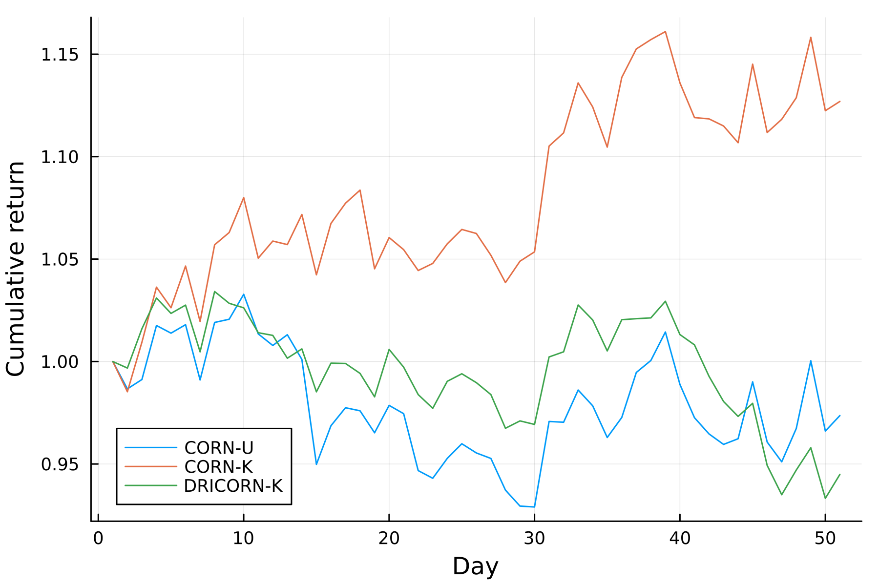
The plot illustrates that the cumulative wealth of CORN-K consistently outperforms the other algorithms. It's important to note that the initial investment for all algorithms is standardized to 1, although this can be adjusted by setting the keyword argument init_budg for each algorithm. Now, let's delve into the performance analysis of the algorithms using prominent performance metrics:
julia> all_metrics = opsmetrics.([m_corn_u.b, m_corn_k.b, m_drcorn_k.b], Ref(rel_pr), Ref(rel_pr_market));Now, one can embed the metrics in a DataFrame and compare the performance of the algorithms with respect to each other:
julia> using DataFrames

julia> nmodels = length(all_metrics);

julia> comp_algs = DataFrame(
           Algorithm = ["CORN-U", "CORN-K", "DRICORN-K"],
           MER = [all_metrics[i].MER for i = 1:nmodels],
           IR = [all_metrics[i].IR for i = 1:nmodels],
           APY = [all_metrics[i].APY for i = 1:nmodels],
           Ann_Sharpe = [all_metrics[i].Ann_Sharpe for i = 1:nmodels],
           Ann_Std = [all_metrics[i].Ann_Std for i = 1:nmodels],
           Calmar = [all_metrics[i].Calmar for i = 1:nmodels],
           MDD = [all_metrics[i].MDD for i = 1:nmodels],
           AT = [all_metrics[i].AT for i = 1:nmodels],
       )
3×9 DataFrame
 Row │ Algorithm  MER        IR         APY        Ann_Sharpe  Ann_Std   Calmar    MDD        AT
     │ String     Float64    Float64    Float64    Float64     Float64   Float64   Float64    Float64
─────┼──────────────────────────────────────────────────────────────────────────────────────────────────
   1 │ CORN-U     0.0514619  0.0963865  -0.126009   -0.505762  0.288691  -1.25383  0.100499   0.847198
   2 │ CORN-K     0.054396   0.198546    0.826495    2.48378   0.324705  17.688    0.0467263  0.87319
   3 │ DRICORN-K  0.0507907  0.0829576  -0.2487     -1.21085   0.22191   -2.54629  0.0976717  0.0053658
The comparison analysis, via comp_algs, highlights that CORN-K outperforms the other algorithms in terms of annualized percentage yield (APY), annualized Sharpe ratio, Calmar ratio, and maximum drawdown (MDD). However, it's essential to note that the annualized standard deviation of CORN-K surpasses that of the other algorithms within this dataset. These individual metrics can be computed separately by using corresponding functions such as sn, mer, ir. For further insights and details, please refer to the Performance evaluation.
References
- B. Li and S. C. Hoi. Online Portfolio Selection: A Survey (2013).