Performance evaluation
This package provides a variety of metrics for evaluating algorithm performance. These metrics are widely recognized in the literature and serve as benchmarks for comparing the performances of different algorithms. Currently, the supported metrics include:
| Row № | Metric | Abbreviation | Direction |
|---|---|---|---|
| 1 | Cumulative Wealth | CW (Also known as $S_n$) | The higher the better |
| 2 | Mean Excess Return | MER | The higher the better |
| 3 | Information Ratio | IR | The higher the better |
| 4 | Annualized Percentage Yield | APY | The higher the better |
| 5 | Annualized Standard Deviation | $\sigma_p$ | The lower the better |
| 6 | Annualized Sharpe Ratio | SR | The higher the better |
| 7 | Maximum Drawdown | MDD | The lower the better |
| 8 | Calmar Ratio | CR | The higher the better |
| 9 | Average Turnover | AT | The lower the better |
Metrics
Cumulative Wealth (CW, Also known as $S_n$)
This metric computes the portfolio's cumulative wealth of the algorithm throughout an investment period. The cumulative wealth is defined as:
\[\begin{aligned} {S_n} = {S_0}\prod\limits_{t = 1}^T {\left\langle {{b_t},{x_t}} \right\rangle } \end{aligned}\]
where $S_0$ represents the initial capital, $b_t$ stands for the portfolio vector at time $t$, and $x_t$ denotes the relative price vector at time $t$. This metric can be evaluated using the sn function.
Mean Excess Return (MER)
MER is utilized to gauge the average excess returns of an OPS method that surpasses the benchmark market strategy. MER is defined as:
\[MER = {1 \over n}\sum\nolimits_{t = 1}^n {{R_t} - } {1 \over n}\sum\nolimits_{t = 1}^n {R_t^*}\]
where $R$ and ${R_t^*}$ represent the daily returns of a portfolio and the market strategy at the $t$th trading day, respectively. For a given OPS method, accounting for transaction costs, ${{R_t}}$ is calculated by ${R_t} = \left( {\mathbf{x}_t\mathbf{b}_t} \right) \times \left( {1 - {\nu \over 2} \times \sum\nolimits_{i = 1}^d {\left| {{b_{t,i}} - {{\tilde b}_{t,i}}} \right|} } \right) - 1$. The market strategy initially allocates capital equally among all assets and remains unchanged. ${R_t^*}$ is defined as: $R_t^* = \mathbf{x}_t \cdot \mathbf{b}^* - 1$ and ${\mathbf{b}^*} = {\left( {{1 \over d},{1 \over d}, \ldots ,{1 \over d}} \right)^ \top }$, where $d$ is the number of assets, and $n$ is the number of trading days. This metric can be calculated using the mer function. (see [25] for more details.)
Information Ratio (IR)
The information ratio is a risk-adjusted excess return metric compared with the market benchmark. It is defined as:
\[IR = \frac{{{{\bar R}_s} - {{\bar R}_m}}}{{\sigma \left( {{R_s} - {R_m}} \right)}}\]
where $R_s$ represents the portfolio's daily return, $R_m$ represents the market's daily return, $\bar R_s$ represents the portfolio's average daily return, $\bar R_m$ represents the market's average daily return, and $\sigma$ represents the standard deviation of the portfolio's daily excess return over the market. Note that in this package, the logarithmic return is used. See ir.
Annualized Percentage Yield (APY)
This metric computes the annualized return of the algorithm throughout the investment period. The annualized return is defined as:
\[\begin{aligned} {APY} = \left( {{S_n}} \right)^{\frac{1}{y}} - 1 \end{aligned}\]
where $y$ represents the number of years in the investment period. This metric can be evaluated using the apy function.
Annualized Standard Deviation ($\sigma_p$)
Another measurement employed to assess risk is the annual standard deviation of portfolio returns. The daily standard deviation is computed to derive the annual standard deviation, after which it is multiplied by $\sqrt{252}$ (assuming 252 days in a year). Users can adjust the number of days in a year by specifying the dpy keyword argument. This metric can be computed using the ann_std function.
Annualized Sharpe Ratio (SR)
The Sharpe ratio serves as a measure of risk-adjusted return. It is defined as:
\[\begin{aligned} SR = {{APY - {R_f}} \over {{\sigma _p}}} \end{aligned}\]
Here, $R_f$ denotes the risk-free rate, typically equivalent to the treasury bill rate at the investment period. This metric can be computed using the ann_sharpe function.
Maximum Drawdown (MDD)
The maximum drawdown is the largest drop percentage of CW from its running maximum over all periods, which looks for the most considerable movement from a peak point to a trough point. Following the definition of Li et al. [19], the maximum drawdown is defined as:
\[MDD = \mathop {\max }\limits_{t \in \left[ {1,T} \right]} \frac{{{M_t} - {S_t}}}{{{M_t}}},\quad {M_t} = \mathop {\max }\limits_{k \in \left[ {1,t} \right]} {S_k}\]
where $M_t$ represents the running maximum of CW, and $S_t$ represents the CW at time $t$. This metric can be calculated using the mdd function.
Calmar Ratio (CR)
The Calmar ratio is a risk-adjusted return metric based on the maximum drawdown. It is defined as:
\[\begin{aligned} CR = {{APY} \over {MDD}} \end{aligned}\]
This metric can be computed using the calmar function.
Average Turnover (AT)
This measure computes how frequently the weight of each asset is changing during the investment period. The lower the AT, the better is performance of the algorithm. The AT can be calculated by:
\[AT = \frac{{{{\sum\nolimits_{t = 2}^T {\left\| {{{\mathbf{b}}_t} - {{\hat {\mathbf{b}}}_{t - 1}}} \right\|} }_1}}}{{2\left( {T - 1} \right)}}\]
where $T$ represents the number of investing days, ${{{\hat {\mathbf{b}}}_{t - 1}}}$ denotes the adjusted portfolio at the end of the $(t − 1)$-th day, which can be calculated using ${\hat {\mathbf{b}}_{t - 1}} = \frac{{{\mathbf{x}_{t - 1}} \odot {\mathbf{b}_{t - 1}}}}{{{\mathbf{x}_{t - 1}}^ \top {\mathbf{b}_{t - 1}}}}$ in which ${{{\mathbf{x}}_{t - 1}}}$ is the price relative vector at time period $t-1$, and ${\left\| \cdot \right\|_1}$ is the L1-norm operator. This metric can be calculated using the at function.
It's noteworthy that these metrics can be computed collectively rather than individually. This can be achieved using the opsmetrics function. This function yields an object of type OPSMetrics containing all the aforementioned metrics.
Examples
Below is a simple example that illustrates how to utilize the metrics. Initially, I utilize the opsmetrics function to compute all the metrics collectively. Subsequently, I present the procedure to compute each metric individually.
opsmetrics function
The opsmetrics function facilitates the computation of all metrics simultaneously. It requires the following positional arguments:
weights: A matrix sized $m \times t$, representing the portfolio weights on each trading day utilizing the chosen OPS algorithm.rel_pr: A matrix sized $m \times t$, which includes the relative prices of assets on each trading day. Typically, these prices are computed as $\frac{p_{t,i}}{p_{t-1,i}}$ in most studies, where $p_{t,i}$ denotes the price of asset $i$ at time $t$. Alternatively, in some studies, relative prices are calculated as $\frac{c_{t,i}}{o_{t,i}}$, where $c_{t,i}$ and $o_{t,i}$ are the closing and opening prices of asset $i$ at time $t$. The user can decide which relative prices to employ and input the corresponding matrix into the function.rel_pr_market: A vector sized $t$, which includes the relative prices of the market benchmark on each trading day. The relative prices of the market benchmark are computed similarly to the relative prices of assets. Note that the function takes the lasttvalues of the vector ifrel_pr_marketcontaints more thantvalues.
Additionally, the function accepts the following keyword arguments:
init_inv=1.: The initial investment, which is set to1.0by default.RF=0.02: The risk-free rate, which is set to0.02by default.dpy=252: The number of days in a year, which is set to252days by default.v=0.: The transaction cost rate, which is set to0.0by default.
The function returns an object of type OPSMetrics containing all the metrics as fields. Now, let's choose few algorithms and assess their performance using the aforementioned function.
julia> using OnlinePortfolioSelection, YFinance, StatsPlots

# Fetch data
julia> tickers = ["AAPL", "MSFT", "AMZN", "META", "GOOG"];

julia> startdt, enddt = "2023-04-01", "2023-08-27";

julia> querry = [get_prices(ticker, startdt=startdt, enddt=enddt)["adjclose"] for ticker in tickers];

julia> prices = stack(querry) |> permutedims;

julia> market = get_prices("^GSPC", startdt=startdt, enddt=enddt)["adjclose"];

julia> rel_pr = prices[:, 2:end]./prices[:, 1:end-1];

julia> rel_pr_market = market[2:end]./market[1:end-1];

julia> nassets, ndays = size(rel_pr);

# Run algorithms for 30 days
julia> horizon = 30;

# Run models on the given data
julia> loadm = load(prices, 0.5, 8, horizon, 0.1);
julia> uniformm = uniform(nassets, horizon);
julia> cornkm = cornk(prices, horizon, 5, 5, 10, progress=true);
┣████████████████████████████████████████┫ 100.0% |30/30

julia> names = ["LOAD", "UNIFORM", "CORNK"];

julia> metrics = (:Sn, :MER, :IR, :APY, :Ann_Std, :Ann_Sharpe, :MDD, :Calmar);

julia> all_metrics_vals = opsmetrics.([loadm.b, uniformm.b, cornkm.b], Ref(rel_pr), Ref(rel_pr_market));

# Draw a bar plot to depict the values of each metric for each algorithm
julia> groupedbar(
         vcat([repeat([String(metric)], length(names)) for metric in metrics]...),
         [getfield(result, metric) |> last for metric in metrics for result in all_metrics_vals],
         group=repeat(names, length(metrics)),
         dpi=300
       )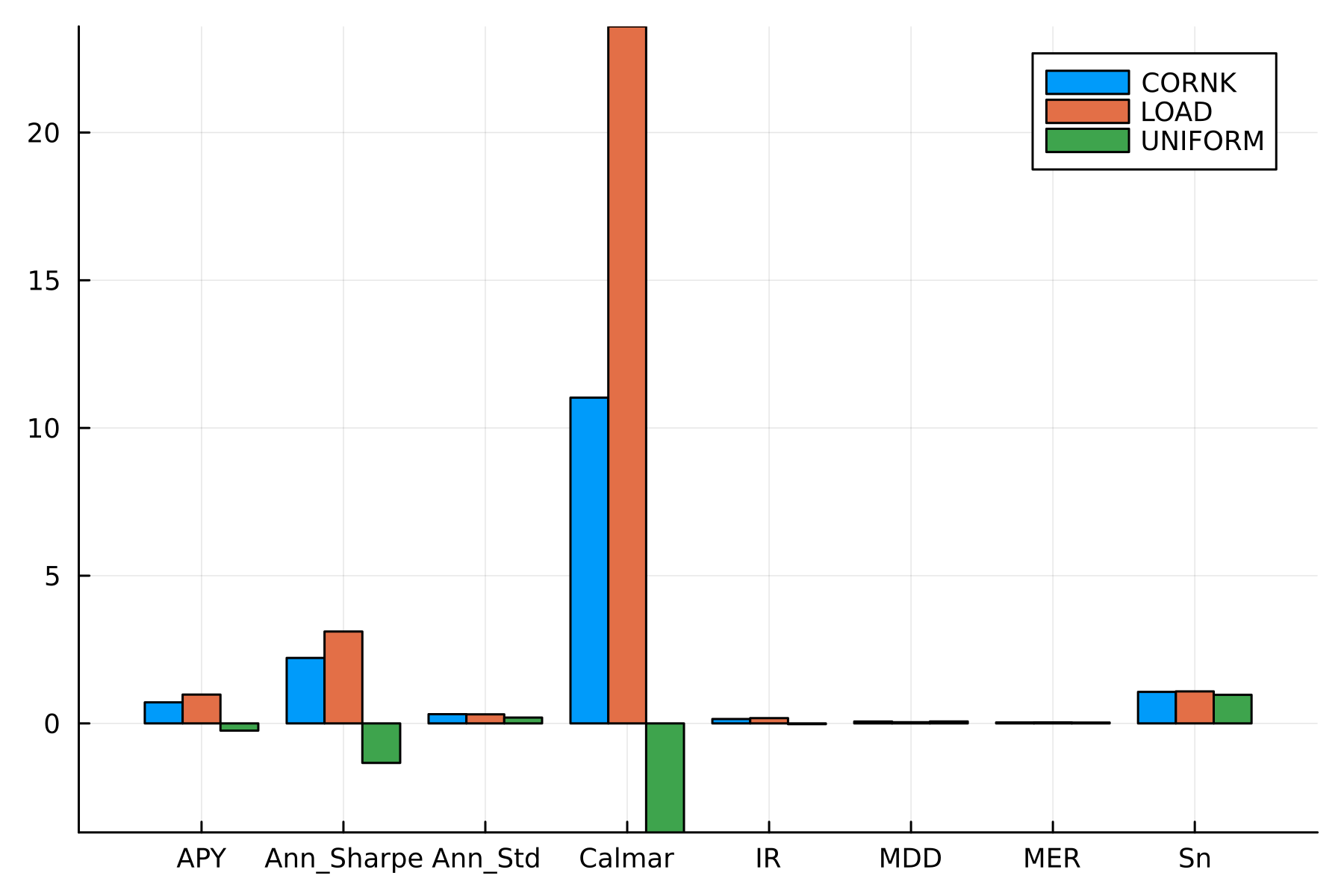
The plot illustrates the value of each metric for each algorithm.
Individual functions
The metrics can be calculated individually as well. For instance, in the next code block, I compute each metric individually for the 'CORNK' algorithm.
# Compute the cumulative wealth
julia> sn_ = sn(cornkm.b, rel_pr)
31-element Vector{Float64}:
 1.0
 1.0056658141861143
 1.0456910599891474
 ⋮
 1.0812597940398256
 1.0561895221684217
 1.0661252685319844

# Compute the mean excess return
julia> mer(cornkm.b, rel_pr)
0.0331885901993342

# Compute the information ratio
julia> ir(cornkm.b, rel_pr, rel_pr_market)
0.14797935671154802

# Compute the annualized return
julia> apy_ = apy(last(sn_), size(cornkm.b, 2))
0.7123367957886144

# Compute the annualized standard deviation
julia> ann_std_ = ann_std(sn_, dpy=252)
0.312367085936459

# Compute the annualized sharpe ratio
julia> rf = 0.02
julia> ann_sharpe(apy_, rf, ann_std_)
2.216420445556956

# Compute the maximum drawdown
julia> mdd_ = mdd(sn_)
0.06460283126873347

# Compute the calmar ratio
julia> calmar(apy_, mdd_)
11.026402121997583

# Compute the average turnover
julia> at(rel_pr, cornkm.b)
0.5710393403115563 # Meaning that the weight of each asset is changing 57% of the time

julia> last(all_metrics_vals)

            Cumulative Wealth: 1.066125303122296
        Mean Excessive Return: 0.03318859854896919
            Information Ratio: 0.1479792121956763
  Annualized Percentage Yield: 0.7123372624638589
Annualized Standard Deviation: 0.31236709233949556
      Annualized Sharpe Ratio: 2.216421894119991
             Maximum Drawdown: 0.06460283279345515
                 Calmar Ratio: 11.026409085516526
             Average Turnover: 0.5710393403115563
As shown, the results are consistent with the results obtained using the opsmetrics function. Individual functions can be found in Functions (see sn, mer, ir, apy, ann_std, ann_sharpe, mdd, calmar, and at for more information).
Tests
In order to investigate whether there are significant differences between some algorithms or not, a statistical analysis can be performed in which, a hypothesis test is considered for paired samples. In this hypothesis test, the difference between the paired samples is the target parameter in which, the paired samples are the APY of two algorithms applied on different datasets [24]. Suppose you want to compare the performance of EG, EGM, and ONS algorithms:
You have to install and import the HypothesisTests.jl package to use this function. One can install the aformentioned package using the following command in Julia REPL:
pkg> add HypothesisTestsjulia> using OnlinePortfolioSelection, HypothesisTests
# Vector of apy values for 3 datasets. I.e. apy value for EG algorithm for Dataset1 is 0.864
julia> apy_EG = [0.864, 0.04, 0.98];
julia> apy_WAEG = [0.754, 0.923, 0.123];
julia> apy_MAEG = [0.512, 0.143, 0.0026];
julia> apy_load = [0.952, 0.256, 0.156];
julia> apys = [apy_EG, apy_WAEG, apy_MAEG, apy_load];
julia> ttest(apys)
4×4 Matrix{Float64}:
0.0 0.960744 0.321744 0.649426
0.0 0.0 0.201017 0.638612
0.0 0.0 0.0 0.14941
0.0 0.0 0.0 0.0The lower the p-values, the better is the performance. The returned matrix by ttest function is a square matrix in which the rows and columns represent the algorithms and the values represent the p-values of t-student test between each pair of algorithms. According to the output above, the performance of the "MAEG" algorithm dominates the "LOAD" algorithm.
To evaluate if the return of the proposed strategy could be due to simple luck, a statistical test can be conducted to measure the probability of this occurrence [33]. It is possible to use the aformentioned ttest function to validate the rubustness of a trading algorithm. The following snippet code provides an example in this regard:
You have to install the GLM.jl package using the following command in Julia REPL:
pkg> add GLMjulia> using OnlinePortfolioSelection, GLM, YFinance
julia> benchmark_prices = get_prices("^GSPC", startdt="2020-02-01", enddt="2020-02-29")["adjclose"]
julia> benchmark_return = benchmark_prices[2:end]./benchmark_prices[1:end-1]
julia> portfolio_return = rand(0.9:1e-5:1.1, length(benchmark_return))
julia> daily_riskfree_return = 1.000156
julia> ttest(benchmark_return, portfolio_return, daily_riskfree_return)
StatsModels.TableRegressionModel{LinearModel{GLM.LmResp{Vector{Float64}}, GLM.DensePredChol{Float64, LinearAlgebra.CholeskyPivoted{Float64, Matrix{Float64}, Vector{Int64}}}}, Matrix{Float64}}
y ~ 1 + x
Coefficients:
────────────────────────────────────────────────────────────────────────────
Coef. Std. Error t Pr(>|t|) Lower 95% Upper 95%
────────────────────────────────────────────────────────────────────────────
(Intercept) -0.0224706 0.0117695 -1.91 0.0743 -0.0474209 0.00247968
x -0.0860158 0.724261 -0.12 0.9069 -1.62138 1.44935
────────────────────────────────────────────────────────────────────────────By analysing the table above, we can conclude that the returns gained by the algorithm are likely to be obtained by chance.
References
- [19]
- Y. Li, X. Zheng, C. Chen, J. Wang and S. Xu. Exponential Gradient with Momentum for Online Portfolio Selection. Expert Systems with Applications 187, 115889 (2022).
- [24]
- M. Khedmati and P. Azin. An online portfolio selection algorithm using clustering approaches and considering transaction costs. Expert Systems with Applications 159, 113546 (2020).
- [25]
- W. Xi, Z. Li, X. Song and H. Ning. Online portfolio selection with predictive instantaneous risk assessment. Pattern Recognition 144, 109872 (2023).
- [33]
- D. Huang, S. Yu, B. Li, S. C. Hoi and S. Zhou. Combination Forecasting Reversion Strategy for Online Portfolio Selection. ACM Trans. Intell. Syst. Technol. 9 (2018).